So, this is the second article I’ve written against the TPC-H Benchmark (Part one here). Recently, Amazon announced that their ‘fast, fully managed petabyte-scale data warehouse service’ was available for public consumption. Having finally had some time to play, I thought I’d take it for a spin.
I was able to get a single node cluster up and running pretty quickly, and installed their sample data set easily. You can read how to go about this in their Getting Started Guide.
The initial issue I had with the sample data set was, well, it was pretty small. Ok, it got the concepts over, but I wanted more. I wanted to get an idea of performance and how it compared across the different levels. I wanted more data.
So, I decided to dump my set of test data (1Gb TPC-H, see part 1 for creating this) into it, and covered here is how I did it.
Getting Started
I’m going to assume that you’ve made it through steps 1-4 of the Getting Started guide above (which covers Prerequisites, Launching the Cluster, Security setup and Connecting to the cluster).
Shown below are the statements used to create the TPC-H tables, within the Redshift environment. You’ll need to create a connection to the Redshift environment, use SQL Workbench to connect to it, and copy and paste this into the SQL window.
CREATE TABLE customer(
C_CustKey int ,
C_Name varchar(64) ,
C_Address varchar(64) ,
C_NationKey int ,
C_Phone varchar(64) ,
C_AcctBal decimal(13, 2) ,
C_MktSegment varchar(64) ,
C_Comment varchar(120) ,
skip varchar(64)
);CREATE TABLE lineitem(
L_OrderKey int ,
L_PartKey int ,
L_SuppKey int ,
L_LineNumber int ,
L_Quantity int ,
L_ExtendedPrice decimal(13, 2) ,
L_Discount decimal(13, 2) ,
L_Tax decimal(13, 2) ,
L_ReturnFlag varchar(64) ,
L_LineStatus varchar(64) ,
L_ShipDate datetime ,
L_CommitDate datetime ,
L_ReceiptDate datetime ,
L_ShipInstruct varchar(64) ,
L_ShipMode varchar(64) ,
L_Comment varchar(64) ,
skip varchar(64)
);
CREATE TABLE nation(
N_NationKey int ,
N_Name varchar(64) ,
N_RegionKey int ,
N_Comment varchar(160) ,
skip varchar(64)
);
CREATE TABLE orders(
O_OrderKey int ,
O_CustKey int ,
O_OrderStatus varchar(64) ,
O_TotalPrice decimal(13, 2) ,
O_OrderDate datetime ,
O_OrderPriority varchar(15) ,
O_Clerk varchar(64) ,
O_ShipPriority int ,
O_Comment varchar(80) ,
skip varchar(64)
);CREATE TABLE part(
P_PartKey int ,
P_Name varchar(64) ,
P_Mfgr varchar(64) ,
P_Brand varchar(64) ,
P_Type varchar(64) ,
P_Size int ,
P_Container varchar(64) ,
P_RetailPrice decimal(13, 2) ,
P_Comment varchar(64) ,
skip varchar(64)
);
CREATE TABLE partsupp(
PS_PartKey int ,
PS_SuppKey int ,
PS_AvailQty int ,
PS_SupplyCost decimal(13, 2) ,
PS_Comment varchar(200) ,
skip varchar(64)
);
CREATE TABLE region(
R_RegionKey int ,
R_Name varchar(64) ,
R_Comment varchar(160) ,
skip varchar(64)
);
CREATE TABLE supplier(
S_SuppKey int ,
S_Name varchar(64) ,
S_Address varchar(64) ,
S_NationKey int ,
S_Phone varchar(18) ,
S_AcctBal decimal(13, 2) ,
S_Comment varchar(105) ,
skip varchar(64)
);
Next up, we need to get some data into it. I’ve had a copy of the TPC-H files sitting on my S3 account for a while, so I was hoping to just point Redshift at that (just like the sample code does). This was where I ran into my first issue. There may be an easier way, but I wanted to do it quickly. The problem was that I couldn’t get the S3 URL syntax to work, and this appears to be because my S3 Buckets are sitting in Ireland (EU). The S3 syntax looks to only work if you are using ‘US Standard’ as your S3 storage. I could be wrong, but I’m not an S3 expert.
Anyway, having created an S3 bucket in US Standard, and transferred the files over, I used the following to copy the contents from these files into the tables created in Redshift.
copy customer from ‘s3://oldnick-tpch/customer.tbl’ CREDENTIALS ‘aws_access_key_id=<Your-Access-Key-ID>;aws_secret_access_key=<Your-Secret-Access-Key>’ delimiter ‘|’;
copy orders from ‘s3://oldnick-tpch/orders.tbl’ CREDENTIALS ‘aws_access_key_id=<Your-Access-Key-ID>;aws_secret_access_key=<Your-Secret-Access-Key>’ delimiter ‘|’;
copy lineitem from ‘s3://oldnick-tpch/lineitem.tbl’ CREDENTIALS ‘aws_access_key_id=<Your-Access-Key-ID>;aws_secret_access_key=<Your-Secret-Access-Key>’ delimiter ‘|’;
copy nation from ‘s3://oldnick-tpch/nation.tbl’ CREDENTIALS ‘aws_access_key_id=<Your-Access-Key-ID>;aws_secret_access_key=<Your-Secret-Access-Key>’ delimiter ‘|’;
copy part from ‘s3://oldnick-tpch/part.tbl’ CREDENTIALS ‘aws_access_key_id=<Your-Access-Key-ID>;aws_secret_access_key=<Your-Secret-Access-Key>’ delimiter ‘|’;
copy partsupp from ‘s3://oldnick-tpch/partsupp.tbl’ CREDENTIALS ‘aws_access_key_id=<Your-Access-Key-ID>;aws_secret_access_key=<Your-Secret-Access-Key>’ delimiter ‘|’;
copy region from ‘s3://oldnick-tpch/region.tbl’ CREDENTIALS ‘aws_access_key_id=<Your-Access-Key-ID>;aws_secret_access_key=<Your-Secret-Access-Key>’ delimiter ‘|’;
copy supplier from ‘s3://oldnick-tpch/supplier.tbl’ CREDENTIALS ‘aws_access_key_id=<Your-Access-Key-ID>;aws_secret_access_key=<Your-Secret-Access-Key>’ delimiter ‘|’;
You’ll need to replace <Your-Access-Key-ID> with your Amazon access key and <Your-Secret-Access-Key> with your secret key, though I bet you’d guessed that. Also, note that it’s possible to load from a gzipped file by adding the gzip parameter to the copy statement, though I didn’t discover this till after the load.
After waiting a little while, though not too long, for Redshift to bring the data in from S3, you can use these queries to check the counts.
select count(*) from customer;
select count(*) from orders;
select count(*) from lineitem;
select count(*) from nation;
select count(*) from part;
select count(*) from partsupp;
select count(*) from region;
select count(*) from supplier;
Next, the Developer Guide section covering loading data into Redshift say you should run the following statements after loading. Analyze updates the database statistics, and Vacuum then reclaims storage space.
analyze;
vacuum;
So, there we go, now we’ve got a Redshift cluster running the TPC-H tables. So next I thought I’d do a basic test to compare results.
My test query for this is shown below, and just does some aggregation against the lineitem table (6 million or so rows).
select l_returnflag, l_linestatus, sum(l_quantity) as sum_qty,
sum(l_extendedprice) as sum_base_price, sum(l_extendedprice*(1-l_discount)) as sum_disc_price,
sum(l_extendedprice*(1-l_discount)*(1+l_tax)) as sum_charge, avg(l_quantity) as avg_qty,
avg(l_extendedprice) as avg_price, avg(l_discount) as avg_disc, count(*) as count_order
from lineitem
group by l_returnflag, l_linestatus
order by l_returnflag,l_linestatus;
So I ran this on my laptop (i7, 12 Gb RAM, 512GB SSD) a couple of times, once as a straight query, and once with a Columnstore index on it, cold (after restart) and warm (2nd time).
SQL times are shown based on SET STATISTICS TIME ON times.
Analysing Redshift was interesting. Since I’ve not done much with Postgres-SQL, I had a look through the Redshift documentation to see what is going on. I found an interesting page showing how to determine if a query is running from disk . Working through this I saw that, once I got the query id from the query below, I could get the query details including memory used and times.
Getting the Query Id
select query, elapsed, substring
from svl_qlog
order by query
desc limit 5;
select *
from svl_query_summary
where query = 5931
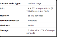
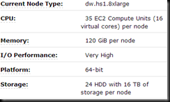
So, having seen those figures, I had a look at the cluster details.
Initially I was using 1 node, so I went up a notch, to a 2 node cluster of the more powerful nodes.
Single Node Testing |
Multi Node Testing |
The Results
| Time to Return (sec) | |
| Laptop – SQL 2012 (Cold) | 24515ms CPU time, 6475ms elapsed |
| Laptop – SQL 2012 (Warm) | 24016ms CPU time, 6060ms elapsed. |
| Laptop – SQL 2102 Columnstore (Cold) | 531ms CPU time, 258ms elapsed |
| Laptop – SQL 2102 Columnstore (Warm) | 389ms CPU time, 112ms elapsed |
| Redshift (1 node cluster) | 1.24 sec |
| Redshift (2 node cluster | 1.4 sec |
So, obviously, I’m not stretching the performance of the Redshift cluster.
Part 2b of this will cover similar tests, though I’ll be doing it with a 100GB TPC-H test data set.
Keep ’em peeled for the next post!


Nick, I want to thank you for this enlightening article, which goes beyond the marketing hype about Redshift. I’m amazed but not surprised: in my personal (and far less scientific tests), I had comparable results. Sure the scale of a Redshift db is not in the GB range, and we should discount network latency from the results, anyway we are talking about a i7 laptop going 4 times faster that a AWS node. I’d definetely go for the laptop 🙂
good job,
Davide
This blog is amazing. I realy like it!
In my tests, scaling from 2*xlarge nodes up to 4*8xlarge nodes gave 10-times improvements in query time. However, I tested with much bigger tables. For a 6 billion row table the time went down from 30 min to 3 min.
Alex Friedgan
Even my team is facing the issue of CPU Utilization going to 100% during loads . In fact the Amazon Redshift Servers goes down when we run our loads .
Is anyone else facing this issue ??
Is anyone having any solution for this issue ???