T-SQL | Dev Blog

Tag Archive: T-SQL

Bringing Twitter into SQL Server – Pt 2 – C#

Filed under: C#, SQL Server — 2 Comments

01/08/2012

Following on from my previous post on bringing data from Twitter into SQL Server, you’ll recall that we were able to take data from a JSON data feed, using cURL, and parse it into SQL Server, using a custom Function.

This enabled the twitter feed to be loaded into a SQL database at the staggering performance of 38 records a second. In a future post, I hope to do some optimisation on the T-SQL process for getting this data in.

However, I wanted to see how quickly the data could be loaded using a C# application (since I’m a bit of a closet coder).

So, following on from Step 1 and Step 2 from the previous post, so you’ve taken the feeds from Twitter, and loaded the data into a Load table in SQL, I then want to get the data into a table in SQL Server.

There are several JSON libraries that are available, that link to C# (a list is here: http://json.org/). I chose JSON.NET (http://json.codeplex.com/) on the basis that it was quite frequently mentioned on StackOverflow (so if I had any questions, I’d stand a reasonable chance of getting an answer), and the examples looked pretty straightforward.

Having fired up VS 2012, I created a project, and added JSON.Net into it using NuGet (I like NuGet!), using Install-Package Newtonsoft.Json.

using System;
using System.Collections.Generic;
using System.Linq;
using Newtonsoft.Json;
using System.Data.SqlClient;

namespace JSONParse
{

class Program
{
static void Main(string[] args)
{
DateTime dStart, dEnd;
dStart = DateTime.Now;

// Connect to SQL
SqlConnection conn = new SqlConnection(“server=localhost; Trusted_Connection=yes; database=twitter_stream;”);
try
{
conn.Open();
}
catch (Exception e)
{
Console.WriteLine(e.ToString());
}

try
{

// Set up the Reader process
SqlDataReader reader = null;
SqlCommand myCommand = new SqlCommand(
“select * from tweetJSON”, conn);
reader = myCommand.ExecuteReader();

while (reader.Read())
{
try
{
// Convert the JSON Data
dynamic obj = JsonConvert.DeserializeObject(reader[1].ToString());
string tJSID = reader[0].ToString();
Console.WriteLine(“id_str {0}”, obj.id_str);
SqlCommand insertcmd = new SqlCommand()
{
CommandText = @”insert into TweetJSONStaging ( tJSID, Country, id_str,
followers_count,profile_image_url,statuses_count,
profile_background_image_url,created_at,friends_count,
location,name,lang, screen_name, source, geo_loc, text)
VALUES (@tJSID, @country,@id_str,@followers, @profileURL, @statuses,
@backgroundimageurl, @created_at, @friendscount,@location, @name,
@lang, @screenname,@source, @geoloc, @text)”
};
insertcmd.Connection = new SqlConnection(“server=localhost; Trusted_Connection=yes; database=twitter_stream;”);
insertcmd.Parameters.AddWithValue(“@tJSID”, tJSID);
insertcmd.Parameters.AddWithValue(“@id_str”, (string)obj.id_str);
insertcmd.Parameters.AddWithValue(“@followers”, (string)obj.user.followers_count);
insertcmd.Parameters.AddWithValue(“@backgroundimageurl”, (string)obj.user.profile_background_image_url);
insertcmd.Parameters.AddWithValue(“@name”, (string)obj.user.name);
insertcmd.Parameters.AddWithValue(“@profileURL”, (string)obj.user.profile_image_url);
insertcmd.Parameters.AddWithValue(“@statuses”, (string)obj.user.statuses_count);
insertcmd.Parameters.AddWithValue(“@friendscount”, (string)obj.user.friends_count);
insertcmd.Parameters.AddWithValue(“@screenname”, (string)obj.user.screen_name);
insertcmd.Parameters.AddWithValue(“@lang”, (string)obj.user.lang);
insertcmd.Parameters.AddWithValue(“@text”, (string)obj.text);
insertcmd.Parameters.AddWithValue(“@source”, (string)obj.source);
insertcmd.Parameters.AddWithValue(“@created_at”, (string)obj.created_at);
string sCountry = “”, sLocation = “”, sGeoloc = “”;

try
{
sCountry = (string)obj.place.country;
}
catch (Exception e)
{
//Console.WriteLine(e.ToString());
}
insertcmd.Parameters.AddWithValue(“@country”, sCountry);

try
{
sLocation = (string)obj.user.location;
}
catch (Exception e)
{
//Console.WriteLine(e.ToString());
}
insertcmd.Parameters.AddWithValue(“@location”, sLocation);
try
{
sGeoloc = String.Join(“,”, obj.place.bounding_box.coordinates.Last.First);
}
catch (Exception e)
{
// Console.WriteLine(e.ToString());
}
insertcmd.Parameters.AddWithValue(“@geoloc”, sGeoloc);

insertcmd.Connection.Open();
try
{
insertcmd.ExecuteNonQuery();
}
catch (Exception)
{ }
insertcmd.Connection.Close();
}
catch (Exception)
{}
}
}
catch (Exception e)
{
Console.WriteLine(e.ToString());
}

dEnd = DateTime.Now;
Console.WriteLine(“Time taken = “+ dEnd.Subtract(dStart));

Console.ReadKey();

}
}
}

Obviously, this code is an example, and you’d be wanting to have proper error handling, better functional layout, better commenting, etc, etc, etc in there, however, you can see how the code runs, and from a performance perspective, it’s better.

Running this code through the Debug mode in Visual Studio, I managed to get 155 records processed a second, pretty snappy.

Then, running it as an Application, outside Visual Studio I got 393 records a second! Just over 10 times faster than T-SQL with a Cursor.

Tags: C#, JSON, Optimisation, SQL Server, T-SQL

Comment

Bringing Twitter into SQL Server – Pt 1 – Basic T-SQL

Filed under: Optimization, SQL Server — 2 Comments

24/07/2012

I’ve been looking at how it might be possible to bring data from Twitter into SQL Server.

You might ask, Why ????

Well, why not ? It’s more an exercise in how this could be done using tools that are available.

There are several steps that I went through, and I’m pretty sure there may be a better way, and if you can think of any improvements, then feel free to use the comments section below.

Step 1 – Getting the Tweets

First up, we need to get the Twitter data. There are numerous ways to do this, however, the easiest way I’ve found is to use a product called cURL (available here: http://curl.haxx.se/download.html).

I saw this referenced while investigating the Microsoft Hadoop on Azure site (https://www.windowsazure.com/en-us/develop/net/tutorials/hadoop-social-web-data/) which was used to extract data to feed into a Hive database.

There are three parts to obtaining the Twitter data using cURL.

Part 1 – Get cURL, you can download this using the link above. I used the Win64 Binary SSL version.

Part 2 – Create a parameters file. As the MS link above shows, the parameters file acts as a filter to get the data you want from the Twitter feed. While it is possible to filter the data by hashtags, I wanted to get a more generalised set of data. To do this, I put the following filter in the parameters file. This effectively filters the data by any tweets that are geotagged.

locations=-180,-90,180,90

Part 3 – Create a batch file to run the job. The batch file created is effectively the same as the one referenced in the MS link. The file is called GetTwitterStream.cmd, and contains the following text. You need to replace <twitterusername> and <twitterpassword> with your twitter credentials.

curl -d @twitter_params.txt -k https://stream.twitter.com/1/statuses/filter.json –u<twitterusername>:<twitterpassword> >>twitter_stream_seq.txt

When you run the GetTwitterStream.cmd file, it starts cURL and starts getting data from the public Twitter streaming API, as shown below.

This gives us a file containing the JSON feed from Twitter.

Step 2 – Load the Twitter JSON Data into SQL

Next we need to get the JSON data from Twitter into SQL. I created a Load table for this, with the following structure:

CREATE TABLE [dbo].[TweetJSON](
[JSONData] [varchar](8000) NULL,
[ID] [int] IDENTITY(1,1) NOT NULL,
[Processed] [char](1) NULL
) ON [PRIMARY]

Then, we can load the JSON file created from cURL in step 1, using BULK INSERT. We need a Format file for this, shown below, and called BIFormatFile.txt

9.0
1
1 SQLCHAR 0 8000 “\r\n” 1 [JSONData] “”

The data can then be loaded using this Bulk Insert task:

BULK INSERT [dbo].[TweetJSON]
from ‘c:\BigData\TwitterData\twitter_stream_seq.txt’
with (CODEPAGE=’RAW’, FORMATFILE=’C:\BigData\twitterdata\BIFormatFile.txt’)

So now, we have a table with the JSON data in, and an Identity column to give us an ID we can reference.

Step 3 – Parse the JSON

Phil Factor has written a great article (here http://www.simple-talk.com/sql/t-sql-programming/consuming-json-strings-in-sql-server/), which covers parsing JSON in T-SQL. I used the parseJSON function from this article, to extract the required fields from the Load table.

I created a staging table:

CREATE TABLE [dbo].[TweetJSONStaging](
[Country] [varchar](200) NULL,
[id_str] [varchar](200) NULL,
[followers_count] [int] NULL,
[profile_image_url] [varchar](200) NULL,
[statuses_count] [int] NULL,
[profile_background_image_url] [varchar](200) NULL,
[created_at] [datetime] NULL,
[friends_count] [int] NULL,
[location] [varchar](200) NULL,
[name] [varchar](200) NULL,
[lang] [varchar](200) NULL,
[screen_name] [varchar](200) NULL,

[varchar](200) NULL,
[geo_lat] [varchar](200) NULL,
[geo_long] [varchar](200) NULL
) ON [Staging]

Then used the following process to iterate through the data and get it into the right format. The process followed here is to create a Cursor (I’ll get to this in a minute) with the records to change, and call the ParseJSON function against it to split the fields out, then to get the fields we want and insert them into a table. Next we set the Processed flag, and repeat the process till there are no more records to process.

declare @JSON NVARCHAR(MAX), @ID int

declare jsCursor CURSOR FOR
select JSONData, ID from tweetJson where Processed is null

open jsCursor

FETCH NEXT from jsCursor into @JSON, @ID
while @@FETCH_STATUS=0
BEGIN
begin try
insert into TweetJSONStaging ( Country, id_str, followers_count,
profile_image_url,statuses_count,profile_background_image_url,created_at,
friends_count,location,name,lang, screen_name, source, geo_lat, geo_long)
select
max(case when NAME=’country’ then StringValue end) as Country,
max(case when NAME=’id_str’ then StringValue end) as id_str,
max(case when NAME=’followers_count’ then convert (int,StringValue) end)
as followers_count,
max(case when NAME=’profile_image_url’ then StringValue end)
as profile_image_url,
max(case when NAME=’statuses_count’ then convert(int,StringValue) end)
as statuses_count,
max(case when NAME=’profile_background_image_url’ then StringValue end)
as profile_background_image_url,
max(case when NAME=’created_at’ then convert(datetime,
(substring (StringValue,9,2)+’ ‘+substring (StringValue,5,3)+’ ‘+
substring (StringValue,27,4) +’ ‘+substring (StringValue,12,2) +’:’+
substring (StringValue,15,2)+’:’+substring (StringValue,18,2) ) ) end)
as created_at,
max(case when NAME=’friends_count’ then convert(int,StringValue) end)
as friends_count,
max(case when NAME=’location’ then StringValue end) as location,
max(case when NAME=’name’ then StringValue end) as name,
max(case when NAME=’lang’ then StringValue end) as lang,
max(case when NAME=’screen_name’ then StringValue end) as screen_name,
max(case when NAME=’source’ then StringValue end) as source,
max(case when element_id=’1′ then StringValue end) as geo_lat,
max(case when element_id=’2′ then StringValue end) as geo_long
from dbo.parseJSON( @JSON)

update tweetJSON
set Processed = ‘Y’
where ID=@ID

end try
begin catch
update tweetJSON
set Processed = ‘X’
where ID=@ID
end catch
FETCH NEXT from jsCursor into @JSON, @ID

end
close jsCursor
deallocate jsCursor

To allow this process to run in a reasonable amount of time, I created a couple of indexes on the load table (tweetJSON). The indexes are on the ID field (Clustered Index) and on the Processed flag.

CREATE UNIQUE CLUSTERED INDEX CI_ID ON [dbo].[TweetJSON]
( [ID] ASC ) ON [PRIMARY]

CREATE NONCLUSTERED INDEX NCI_Processed ON [dbo].[TweetJSON]
( [Processed] ASC ) ON [PRIMARY]

Running this process took approx. 26 seconds to load 1000 records, so approx. 38 records a second.

So, I thought I’d try it with a While clause, rather than a cursor, and interestingly, it took the same amount of time to run, for 1000 records.

Update: As raised by Dave Ballantyne (@davebally), this shows that a While clause is effectively doing the same as the Cursor, since the process is still running over records one by one. (Further information can be found here).

declare @JSON varchar(8000), @ID int, @count int

while 1=1
BEGIN
select top 1 @JSON = JSONData, @ID=ID from tweetJson where Processed =’N’
begin try
insert into TweetJSONStaging ( Country, id_str, followers_count,
profile_image_url,statuses_count,profile_background_image_url,created_at,
friends_count,location,name,lang, screen_name, source, geo_lat, geo_long)
select
max(case when NAME=’country’ then StringValue end) as Country,
max(case when NAME=’id_str’ then StringValue end) as id_str,
max(case when NAME=’followers_count’ then convert (int,StringValue) end)
as followers_count,
max(case when NAME=’profile_image_url’ then StringValue end)
as profile_image_url,
max(case when NAME=’statuses_count’ then convert(int,StringValue) end)
as statuses_count,
max(case when NAME=’profile_background_image_url’ then StringValue end)
as profile_background_image_url,
max(case when NAME=’created_at’ then convert(datetime,
(substring (StringValue,9,2)+’ ‘+substring (StringValue,5,3)+’ ‘+
substring (StringValue,27,4) +’ ‘+substring (StringValue,12,2) +’:’+
substring (StringValue,15,2)+’:’+substring (StringValue,18,2) ) ) end)
as created_at,
max(case when NAME=’friends_count’ then convert(int,StringValue) end)
as friends_count,
max(case when NAME=’location’ then StringValue end) as location,
max(case when NAME=’name’ then StringValue end) as name,
max(case when NAME=’lang’ then StringValue end) as lang,
max(case when NAME=’screen_name’ then StringValue end) as screen_name,
max(case when NAME=’source’ then StringValue end) as source,
max(case when element_id=’1′ then StringValue end) as geo_lat,
max(case when element_id=’2′ then StringValue end) as geo_long
from dbo.parseJSON( @JSON)

update tweetJSON
set Processed = ‘Y’
where ID=@ID

end try
begin catch
update tweetJSON
set Processed = ‘X’
where ID=@ID
end catch

select @count=count(1) from tweetJson where Processed =’N’

if @count=0
break
else
continue
end

Thanks for reading! I’ll add an update when I’ve made changes to make it more performant.

Tags: JSON, SQL Server, T-SQL

Comment

T-SQL Tuesday #32 – A Day in the Life – #TSQL2sday

Standard

Filed under: Community, SQL Server, T-SQL Tuesday — 1 Comment

17/07/2012

Thanks to Erin Stellato for hosting this months #TSQL2sday. Erin wanted to know all about what we do every day!

Interestingly, when I was much younger, I wanted to be a Fire-fighter or a Pilot. I’m still quite keen on learning to fly, but that’s looking less likely as time is going by (Eyesight, time, age and cost in that order).

Now though, and for the past 12 years or so, I work as a Consultant. It’s a nice, vague title. It started out as ‘Technical Consultant’, moved through Systems Consultant, and CRM Consultant. It’s currently bouncing between BI Consultant and Data Warehousing Consultant depending on the project I’m working on.

My Journey to Work

The Office

My Day!

The day started by sitting in a traffic jam. Pretty common that, unfortunately.

However, when I made it to my desk, I did a couple of checks of a server that I was running maintenance jobs on overnight. All was well, so I dived into email.

A couple of interesting items in there, one was a link about a Pigeon with a USB stick being faster than UK broadband (BBC link here). Also, was an invitation to the Microsoft Hadoop on Azure trial, which looks really interesting, and something I’ll have a look at next week (link here).

The Morning

Then, I started work on a Customer project that I’m working on this week. It’s effectively adding two additional country feeds (Spain and France, since you asked), to a data warehouse. The customer is using WhereScape RED, so it was a pretty straightforward matter of dragging and dropping the tables from the DB2 source system, into the ETL tool. WhereScape RED then generates the stored procedures to allow the ETL process to run, to get the data into the DWH.

Sounds a pretty straightforward process, however, there are 91 tables, and a couple of minor modifications to each one. So that took up all of my morning.

The Afternoon

The afternoon was pretty much taken up by an interesting problem with a BusinessObjects (XI4)environment. It was apparently continually running a query against the SQL Server database. We managed to prove it was the BO server doing this by changing the service account it was running as. The query could be seen in sp_whoisactive (thank you @AdamMachanic) to be run by a different user. The query was proceeding to take the server utilisation to 100%, which meant that the other databases on the server couldn’t effectively service user queries.

To temporarily resolve this issue, we put Resource Governor on, which restricted the BusinessObjects service to 25% of the CPU power, thereby letting the other users have some resources.

I found a really helpful query that helped me to find the queries that were being run. The query (from SQLAuthority, is copied here).

SELECT sqltext.TEXT, req.session_id, req.status,req.command, req.cpu_time, req.total_elapsed_time FROM sys.dm_exec_requests req CROSS APPLY sys.dm_exec_sql_text(sql_handle) AS sqltext

Copied from http://blog.sqlauthority.com/2009/01/07/sql-server-find-currently-running-query-t-sql/

The final solution to the issue was to apply the BO XI4 SP4 patch, which appears to have resolved the issue.

There was also a couple of questions on licencing, to which both answers were ‘If it looks to be too good to be true, it probably is’.

Sadly, I didn’t get any pictures of the Red Arrows flying around the Farnborough Airshow, which is just up the road from us, or any pictures of the White-tailed Kite we saw flying over the motorway.

And that, is pretty much my day; a comparatively quiet one, and for a change, I made it out the door and home at a reasonable time. I hope you found this interesting, and I look forward to reading about your day.

Thanks again to Erin for hosting.

Tags: SQL Server, T-SQL

Comment

T-SQL Tuesday #29 – ColumnStore–Faster than a speeding Clustered Index… #TSQL2sDay

Filed under: Community, SQL Server, T-SQL Tuesday — 1 Comment

10/04/2012

It’s T-SQL Tuesday again, and this time hosted by Nigel Sammy. Thanks for hosting Nigel, enjoy the post.

Not so long ago, I was lucky enough to go to SQL Bits X. It was a great few days, an I highly recommend it to you!

The Keynote session, given by Conor Cunningham, was a 400 level session on the ColumnStore index, which is a new feature in SQl Server 2012.

The demo was, unsurprisingly, really good, and it made me wonder ‘is it really that good ?’ So I thought I’d give it a go and see.

Having Googled around a bit, I found a useful blog article by Sacha Tomey, that went through a few examples. With permission, I’m going to run through a similar process, add a few bits in, and use a different data set.

Part of me really hates the AdventureWorks demo database, so you can imagine my delight when I discovered that there is now a bigger Retail data set, structured as a DataWarehouse. This is the Contoso BI set, and I like it.

Getting down to it

After installing the ContosoBI database, you’ll end up with a fact table, factOnlineSales, with approx. 12.6 million rows in it.

First off, I want to try and get a level playing field, so we’ll be running with Statistics IO and Statistics Time on, and we’ll be clearing the buffers before each query

set statistics IO on;
set statistics time on;
dbcc dropcleanbuffers;

The Clustered Index

Just to get a comparison, I ran the test query, shown below, to get an idea of the speed against the supplied Clustered Index.

dbcc dropcleanbuffers;
go
SELECT
StoreKey ,SUM(SalesAmount) AS SalesAmount
FROM factOnlineSales
GROUP BY StoreKey
ORDER BY StoreKey

This gave the following results:

Table ‘Worktable’. Scan count 0, logical reads 0, physical reads 0, read-ahead reads 0, lob logical reads 0, lob physical reads 0, lob read-ahead reads 0.
Table ‘FactOnlineSales’. Scan count 5, logical reads 46821, physical reads 1, read-ahead reads 46532, lob logical reads 0, lob physical reads 0, lob read-ahead reads 0.

SQL Server Execution Times:
CPU time = 8377 ms, elapsed time = 3476 ms

Just a Heap

Next, I wanted to get rid of the Clustered index, but since I didn’t really want to lose the original table, I ran this code to insert the contents of the factOnlineSales table into factCleanSales.

select * into factCleanSales from FactOnlineSales

That gave me 12 million rows, I wanted more, so next I ran this:

insert into factCleanSales
select dateadd(yy,3,DateKey), StoreKey, ProductKey, PromotionKey, CurrencyKey, CustomerKey, SalesOrderNumber, SalesOrderLineNumber, SalesQuantity, SalesAmount,
ReturnQuantity, ReturnAmount, DiscountQuantity, DiscountAmount, TotalCost,
UnitCost, UnitPrice, ETLLoadID, dateadd(yy,3,LoadDate), dateadd(yy,3,UpdateDate) from factOnlineSales

This gave me approx. 25 million records, and no Clustered Index. So I ran the test query again. It took a little longer this time.

dbcc dropcleanbuffers;
go
SELECT
StoreKey ,SUM(SalesAmount) AS SalesAmount
FROM factCleanSales
GROUP BY StoreKey
ORDER BY StoreKey

Table ‘Worktable’. Scan count 0, logical reads 0, physical reads 0, read-ahead reads 0, lob logical reads 0, lob physical reads 0, lob read-ahead reads 0.
Table ‘factCleanSales’. Scan count 5, logical reads 505105, physical reads 0, read-ahead reads 504823, lob logical reads 0, lob physical reads 0, lob read-ahead reads 0.

SQL Server Execution Times:
CPU time = 14976 ms, elapsed time = 33987 ms.

Nearly 10 times longer to run, and more than 10 times the I/O, but that wasn’t surprising since we had no indexes.

Add one Non-Clustered

So, following Sacha’s lead, I added a compressed, nonclustered index into the pot.

CREATE NONCLUSTERED INDEX [IX_StoreKey] ON [dbo].factCleanSales
( StoreKey ASC )
INCLUDE ([SalesAmount]) WITH
(
PAD_INDEX = OFF, STATISTICS_NORECOMPUTE = OFF, SORT_IN_TEMPDB = OFF, DROP_EXISTING = OFF, ONLINE = OFF, ALLOW_ROW_LOCKS = ON,
ALLOW_PAGE_LOCKS = ON, FILLFACTOR = 100, DATA_COMPRESSION = PAGE
) ON [PRIMARY]
GO

Clearing the buffers and running the query now, resulted in a better experience.

Table ‘factCleanSales’. Scan count 5, logical reads 43144, physical reads 1, read-ahead reads 42999, lob logical reads 0, lob physical reads 0, lob read-ahead reads 0.

SQL Server Execution Times:
CPU time = 18877 ms, elapsed time = 5785 ms.

The query time was down to a more reasonable level, though still longer than the Clustered Index.

ColumnStore Time!

Adding the ColumnStore index took a while, just over 2 minutes. The definition is below, so I ran it. Note that the ColumnStore index has all the columns in the definition. You can’t have Include Columns, and by having all the columns in there, you gain huge flexibility for the Index.

Create nonclustered columnstore index [IX_ColumnStore] on [dbo].factCleanSales
( OnlineSalesKey, DateKey, StoreKey, ProductKey,
PromotionKey, CurrencyKey, CustomerKey, SalesOrderNumber,
SalesOrderLineNumber, SalesQuantity, SalesAmount, ReturnQuantity,
ReturnAmount, DiscountQuantity, DiscountAmount, TotalCost, UnitCost,
UnitPrice, ETLLoadID, LoadDate, UpdateDate
) with (Drop_Existing = OFF) on [PRIMARY];

Next I ran the test query.

Table ‘factCleanSales’. Scan count 4, logical reads 6378, physical reads 27, read-ahead reads 13347, lob logical reads 0, lob physical reads 0, lob read-ahead reads 0.
Table ‘Worktable’. Scan count 0, logical reads 0, physical reads 0, read-ahead reads 0, lob logical reads 0, lob physical reads 0, lob read-ahead reads 0.

SQL Server Execution Times:
CPU time = 515 ms, elapsed time = 378 ms.

That’s less than a tenth of the time the Clustered index took, and the great thing is, because it’s got all the columns in there, you can create more complicated queries, and still get amazing speed. By running the query below, we still got great speed!

dbcc dropcleanbuffers;
go
SELECT
year(DateKey), storekey ,SUM(SalesAmount) AS SalesAmount
FROM factCleanSales with (index ([IX_ColumnStore]))
GROUP BY year(DateKey), storekey
ORDER BY year(DateKey)

Table ‘factCleanSales’. Scan count 4, logical reads 8156, physical reads 78, read-ahead reads 16224, lob logical reads 0, lob physical reads 0, lob read-ahead reads 0.
Table ‘Worktable’. Scan count 0, logical reads 0, physical reads 0, read-ahead reads 0, lob logical reads 0, lob physical reads 0, lob read-ahead reads 0.

SQL Server Execution Times:
CPU time = 4603 ms, elapsed time = 1522 ms.

Is there a Downside ?

Yes. Two actually.

Firstly, it’s an Enterprise only feature. This is annoying, however, it is linked to the second downside. You cannot insert, update or delete directly, when a ColumnStore index is present.

Msg 35330, Level 15, State 1, Line 1
UPDATE statement failed because data cannot be updated in a table with a columnstore index. Consider disabling the columnstore index before issuing the UPDATE statement, then rebuilding the columnstore index after UPDATE is complete.

This means that if you are using it on a Data Warehouse, you’ll need to disable the index on the fact table, insert/update the data, then rebuild the index to get it back online. This isn’t ideal, however, there is an alternative. You can use Partition Switching to switch data in and out of the table.

Effectively, what you’ll be doing to insert data, is to load data into a partition table, with the same schema as the fact table, and switch it in. For updating or deleteing, you’d switch the appropriate partition out, update/delete the data, then switch it back in again. It’s more complicated (obviously), but the performance improvement gained by ColumnStore indexes should be worth it. Given that Table Partitioning is an Enterprise feature, it makes sense (kind of) that ColumnStore indexes should be too.

Partition Switching

To demonstrate how inserting into a table with a ColumnStore index on it was working, I dropped the indexes against the factCleanSales table, and partitioned and clustered it using the following:

CREATE PARTITION FUNCTION [myPartFunc](int) AS RANGE RIGHT
FOR VALUES (N’2003′, N’2004′, N’2005′, N’2006′, N’2007′, N’2008′, N’2009′,
N’2010′, N’2011′, N’2012′, N’2013′, N’2014′, N’2015′)

CREATE PARTITION SCHEME [myPartScheme] AS PARTITION [myPartFunc] TO
([PRIMARY], [PRIMARY], [PRIMARY], [PRIMARY], [PRIMARY], [PRIMARY],
[PRIMARY], [PRIMARY], [PRIMARY], [PRIMARY], [PRIMARY], [PRIMARY],
[PRIMARY], [PRIMARY])

CREATE CLUSTERED INDEX [ClusteredIndex_on_myPartScheme_634694274321586358] ON [dbo].[factCleanSales]
( [YearPart] )WITH (SORT_IN_TEMPDB = OFF, DROP_EXISTING = OFF, ONLINE = OFF) ON [myPartScheme]([YearPart])

Then, added the ColumnStore back into the table, and this is automatically matched to the Partitioning function and scheme above.

CREATE NONCLUSTERED COLUMNSTORE INDEX [IX_ColumnStore] ON [dbo].[factCleanSales] ( [OnlineSalesKey], [DateKey], [StoreKey], [ProductKey], [PromotionKey], [CurrencyKey], [CustomerKey], [SalesOrderNumber], [SalesOrderLineNumber], [SalesQuantity], [SalesAmount], [ReturnQuantity], [ReturnAmount], [DiscountQuantity], [DiscountAmount], [TotalCost], [UnitCost],
[UnitPrice], [ETLLoadID], [LoadDate], [UpdateDate], [YearPart]
)WITH (DROP_EXISTING = OFF)

Next, I created a table to switch the data in from, then loading it up, adding the ColumnStore index, and then switching the partition in using this:

CREATE TABLE [dbo].[factCleanSales_Part](
[OnlineSalesKey] [int] IDENTITY(1,1) NOT NULL,
[DateKey] [datetime] NOT NULL,
[StoreKey] [int] NOT NULL,
[ProductKey] [int] NOT NULL,
[PromotionKey] [int] NOT NULL,
[CurrencyKey] [int] NOT NULL,
[CustomerKey] [int] NOT NULL,
[SalesOrderNumber] [nvarchar](20) NOT NULL,
[SalesOrderLineNumber] [int] NULL,
[SalesQuantity] [int] NOT NULL,
[SalesAmount] [money] NOT NULL,
[ReturnQuantity] [int] NOT NULL,
[ReturnAmount] [money] NULL,
[DiscountQuantity] [int] NULL,
[DiscountAmount] [money] NULL,
[TotalCost] [money] NOT NULL,
[UnitCost] [money] NULL,
[UnitPrice] [money] NULL,
[ETLLoadID] [int] NULL,
[LoadDate] [datetime] NULL,
[UpdateDate] [datetime] NULL,
[YearPart] [int] NULL
)

alter table [factCleanSales_Part] with check add constraint chk2006 check (yearPart=2006)

CREATE CLUSTERED INDEX [ClusteredIndex_on_myPartScheme_634694274321586358] ON [dbo].[factCleanSales_Part] ( [YearPart]
)WITH (SORT_IN_TEMPDB = OFF, DROP_EXISTING = OFF, ONLINE = OFF) ON [myPartScheme]([YearPart])

insert into factCleanSales_Part
select dateadd(yy,-1,DateKey), StoreKey, ProductKey, PromotionKey, CurrencyKey, CustomerKey, SalesOrderNumber, SalesOrderLineNumber, SalesQuantity, SalesAmount,
ReturnQuantity, ReturnAmount, DiscountQuantity, DiscountAmount, TotalCost,
UnitCost, UnitPrice, ETLLoadID, dateadd(yy,-1,LoadDate),
dateadd(yy,-1,UpdateDate) , year(dateadd(yy,-1,DateKey)) from factOnlineSales
where year(dateadd(yy,-1,DateKey))=2006

CREATE NONCLUSTERED COLUMNSTORE INDEX [IX_ColumnStore] ON [dbo].factCleanSales_Part (
[OnlineSalesKey],    [DateKey],    [StoreKey],    [ProductKey],    [PromotionKey],
[CurrencyKey],    [CustomerKey],    [SalesOrderNumber],    [SalesOrderLineNumber],
[SalesQuantity],    [SalesAmount],    [ReturnQuantity],    [ReturnAmount],
[DiscountQuantity],    [DiscountAmount],    [TotalCost],    [UnitCost],
[UnitPrice],    [ETLLoadID],    [LoadDate],    [UpdateDate],    [YearPart]
)WITH (DROP_EXISTING = OFF)

Next, to check that there are no records in the partition already for 2006, I ran this:

SELECT YearPart, $PARTITION.myPartFunc(YearPart) AS Partition,
COUNT(*) AS [COUNT] FROM factCleanSales
GROUP BY YearPart, $PARTITION.myPartFunc(YearPart)
ORDER BY Partition

Next, I switched the data in using this, and then checked the partition values using the statement above.

alter table [factCleanSales_Part] with check add constraint chk2006 check (yearPart=2006)

Delightfully, the fact table now has another partition, and all without removing the ColumnStore index on it.

For Extra credit…

Now, should you want to get more details out of the columnstore index, there are a couple of new DMV’s that can be used. They are:

sys.column_store_dictionaries
sys.column_store_segments

To see useful information like the sizing or number of rows per column, you can use this query:

select object_name(p.object_id) as ‘TableName’, p.partition_number,p.data_compression_desc,
c.name, csd.entry_count, csd.on_disk_size
from sys.column_store_dictionaries csd
join sys.partitions p on p.partition_id = csd.partition_id
join sys.columns c on c.object_id = p.object_id and c.column_id= csd.column_id
order by p.partition_number, c.column_id

which will return the following data. Summing the on_disk_size will give you the size in bytes of the index.

My Demo Environment

Just for transparency, the timings I was getting above weren’t on any huge server. They were on a virtual machine, running in VMWare Workstation v8.0.2 on Windows 7 SP1. SQL Server is 2012 (obviously), Developer Edition in 64bit.

Wrapping up..

I think it’s reasonably safe to say that this is the longest (in size and time) blog post I’ve written, so I apologise if it rambles a bit, but I hope you get the importance of ColumnStore indexes, and I hope you get the chance to use them.

Tags: SQL Server, T-SQL, TSQL

Comment

Presenting in Spring… #sqlserver #sqlclr

Filed under: C#, C++, Community, SQL Server — Leave a comment

02/04/2012

Having been sitting on the fence for a while, I’m finally leaping off, and presenting at some community events. Following a false start with SQLBits (I submitted, but wasn’t voted in, and given the number of attendees I’m a little relieved about that!), I’ll be presenting at the following events over the next couple of months.

Hope to see you there!

24^th April (Tues) – SQL Server in the Evening (6:30-6:50) – First Timers Slot (http://sqlserverfaq.com/events/392/Sessions-including-SQL-Server-Parallel-Data-Warehouse-at-the-sixth-SQL-Server-community-event-615pm-April-24th-Reading-Berkshire.aspx)

I’ll talk about using the CLR within SQL Server, why and when it should be used and then how.

25^th April (Weds) – DevEvening (http://www.devevening.co.uk/)

26^th May (Sat)– DDD Southwest (http://dddsouthwest.com/)
NOTE: This session isn’t confirmed yet, and is still reliant on being voted in. You can vote by going to the DDD Southwest site, linked above! )

Both DevEvening and DDD Southwest will be the same session, summarised below:

Going Native with SQL Server 2012 and C++

I’ll be going through the delights of creating a module to interact with SQL Server 2012, a function in T-SQL (briefly), then using C# to create a SQL CLR module, and then looking into the performance gains by making a C++ application querying the SQL Native Client (ODBC). All three sections will do the same job, and we’ll cover the advantages and disadvantages of each.

We’ll cover the following:

T-SQL, SQL CLR (C#)
SQL Server Native Client
Advantages and Disadvantages
Performance Opportunities
How to use it to connect to SQL Server from C++
How to query a database
Comparison between T-SQL, SQL CLR & C++ solutions

Slides and follow-up articles will be coming soon.

Tags: CLR, SQL Server, T-SQL

Comment

T-SQL Tuesday #28–See the Obvious – #TSQL2sDay

Filed under: T-SQL Tuesday, Thoughts — 1 Comment

13/03/2012

Thanks to Argenis Fernandez for hosting this month.

A Random Start

I’ve had an interesting (I hope) experience in my career this far. I started out, working in a Pharmacy.. It was back there that I wrote my first computer program, well actually it was at college, but it was for them. Many eons ago, back in the early 90’s, I’d been learning Pascal at college, and things are easier to learn, if you have an aim, so I wrote a program to assist will the filling in of paperwork. It worked, and it was good. It stored data in a pipe-delimited file, rather than any kind of database. Not good, for many reasons, but it was only a single user application, and didn’t have a huge amount of data.

Know your limits…

After that, I went to university, where they tried to teach me C++, assembly and Haskell. They failed with assembly and Haskell, though the theory is still there. C++ I love, and keep going back to. In fact, with any luck, you may see me present on it at DDD Southwest in May, and at DevEvening in April… Sadly, while I do enjoy C++, I’m not good enough to do that as a career, and I don’t think I’d enjoy it as much if it was my bread+butter.

Part of the Degree I did (Computer Systems, since you asked) included a year work placement. I did this at a small IT Company, where I worked on the Support Desk. This was a pretty small company, so while I did Application support for customers, I also managed the internal infrastructure, created their website and a few other bits. It was a great experience and I really enjoyed it. So much so, that I went back there to do consultancy after I’d completed the degree.

While I was there, I learnt Windows NT, Visual Basic, Btrieve and had my first introductions to SQL Server (6.5 and 7). It was also here that I took my first Microsoft Certifications, covering Windows NT, SQL Server and assorted Networking topics.

Know when it’s time to move

After four years, I was starting to feel claustrophobic, and needed more of a challenge. At the start of 2000, I moved on, and went to work for a Siebel Consultancy. This was a big change, as while I’d done some consultancy work before, I really had to up my game. Not a bad thing, and I really found my feet with Siebel as it was based on SQL Server, and had the ability to have custom components written in Siebel VB or eScript.

More Certifications

After a great couple of years, with big Siebel implementations, including a great system linking Siebel to SAP, via XML integrations (my first real experience with enterprise-grade XML), the Siebel market for us dropped off after Oracle bought Siebel ($5.8 Billion!).

I then moved my skills to Microsoft CRM, starting with V1.2 (unpleasant), then v3.0 (much better), and also SharePoint, all of which had associated MS Certifications which I completed, and all of which were based on SQL Server.

Try to see the Obvious…

At some point, and I can’t remember when, I realised that I’d been working with SQL Server, for over 12 years, and now it’s nearing 15. I hadn’t really noticed.

For the past two years I’ve been working as a Consultant, building Data Warehouses primarily, though I also do some C# for SQL CLR work, and C++ for fun. I’ve done a ridiculous number of Certifications (mostly Microsoft) and, my motivation is to get validation of my skills. I’m working on the MCM: SQL Server certification at the moment, and have the final Lab exam in May.

What Next ?

I don’t know. I’m pretty sure there will be SQL Server involved though. Fortunately the new version of SQL Server is out now, so the new Certifications will be out soon, and that’ll keep me occupied for a while.

From reading this though, the one thing that strikes me, is that I’ve been very lucky to be in a career that keeps my brain occupied. If there are less taxing times, then I have C++ to stretch the grey matter.

One other thing; I’ve also found that it is good to keep pushing yourself. Always try to work just outside your comfort zone. If everything is easy, then you need to push yourself more.

To end, a couple of thoughts from wiser people than me.

Tags: SQL Server, T-SQL

Comment

Loading Reference Data from a SharePoint List using SSIS

Filed under: SharePoint, SQL Server — 5 Comments

26/01/2012

Recently, I’ve been working on a project where the reference data is stored in SharePoint lists. While it is possible to get the information out of the SQL Server database directly, using something like the T-SQL below, it’s a bit messy.

SELECT      dbo.UserData.tp_ID,
   dbo.UserData.tp_ListId,
   dbo.UserData.tp_Author,
   dbo.UserData.nvarchar1,
   dbo.UserData.nvarchar2,
   dbo.UserData.nvarchar3
FROM            dbo.Lists
INNER JOIN
                 dbo.UserData ON dbo.Lists.tp_ID = dbo.UserData.tp_ListId
WHERE    (dbo.Lists.tp_title like 'TestList')


I wasn’t able to use this to get the data out, as the client doesn’t allow direct access to the SharePoint database, which is entirely reasonable, given that it’s their corporate intranet.

To get around this, I found a very useful set of additional modules for Integration Services (http://sqlsrvintegrationsrv.codeplex.com/), one of which is a SharePoint List Source and Destination. These then allow you to read the data directly.

Using the SharePoint List Source & Destinations

1. The first step is to download the SharePoint List Source and Destination module from http://sqlsrvintegrationsrv.codeplex.com/, and install it.

2. Having done that, you need to start up BIDS (BI Development Studio / VS 2008) and create an ‘Integration Services Package’.

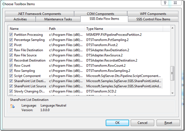
3. You’ll need to add the two new Data flow items into the Toolbox (in Tools > Choose Toolbox Items, in the SSIS Data Flow Items section)

4. Add a Dataflow Task to the Control Flow in the SSIS Package.

5. Right click on the Connection Manager Section at the bottom of the Control Flow, and choose SPCRED (Connection Manager for SharePoint Connections). Click OK, when the Dialog for the SharePoint Connection opens.

6. Then drill into the Data Flow Task, to take you to the Data Flow. In there, drag in a SharePoint List Source

7. Right click on the List Source, choose Show Advanced Editor. In the Connection Managers tab, pick the SharePoint Connection you created in step 5.

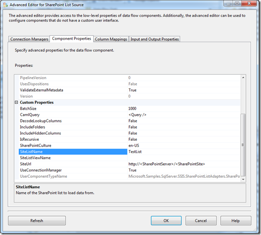
8. Next, click on the Component Properties tab. In this tab, you need to specify the Name of your SharePoint list (SiteListName) and the URL of your SharePoint server (SiteUrl). The SiteUrl is the Parent site within which your List appears. If you want to filter the information from SharePoint, you can modify the CamlQuery section in here, and add a SharePoint CAML query.

9. Once you’ve populated this, click on Refresh, and if everything is working, you’ll be able to move to the next tab. If there are errors (such as an incorrect SiteUrl), you’ll get errors like the one below.

10. Moving on to the Column Mappings tab, then gives you a list of fields and mappings, representing the Available fields from SharePoint (on the left) and fields that will be available to pass out of the List Source (on the right). You can remove fields that are not relevant here, if you’d like, then click Ok, to return to the Data Flow.

11. We need to add an OLE DB Connection manager, by right clicking Connection Managers at the bottom, and choosing ‘New OLE DB Connection’.

12. To get the SharePoint list contents into a database table, we need to add an OLE DB Destination, so drag that into the Data Flow and hook the Green output from the SharePoint List Source to the top of the OLE DB Destination. You’ll then see that there is a red X on the OLE DB Destination, so we need to make some changes.

13. Since we need to make changes to the OLE DB Destination, double click on the OLE DB Destination. As shown below, we need to specify a table for the SharePoint data to go to. The drop down list has a list of the tables in the database connected to the OLE DB Connection Manager, so pick a table (if you’ve made one already) or click new to create a new table.

14. Then click ‘Mappings’ on the left, and it’s possible to link the field in the source (SharePoint List) to your destination table.

15. You’ll then be able to run this SSIS Package, and assuming all is running successfully, you’ll see green boxes.

NOTE: Any text fields that are stored in SharePoint Lists, are stored as Unicode strings in the database (so nvarchar).

Further documentation on using these adapters is available here.

Tags: SharePoint, SQL Server, SSIS, T-SQL

Comment

Partitioning in SQL Server

Filed under: Optimization, SQL Server — Leave a comment

22/08/2011

During the my preparation for the 70-451 Certification, I did some work on Partitioning. I found this to be quite an interesting exercise, so wanted to share it.

There are a number of reasons that you could do Partitioning, though primarily they are related to performance, and easier maintenance. However, while you can get an increase in performance, it isn’t the answer to all your problems.

The performance gain is through the ability to have a database table spread over multiple I/O devices (through filegroups), though this also gives you the ability to do partial database restores.

Step 1 – Create a database

The First step, is obviously to create a database to play with.

CREATE DATABASE [sandpit] ON  PRIMARY
( NAME = N'sandpit', FILENAME = N'C:\temp\sandpit.mdf' , SIZE = 200mb ,
   MAXSIZE = UNLIMITED, FILEGROWTH = 256000KB )
 LOG ON
( NAME = N'sandpit_log', FILENAME = N'C:\temp\sandpit_log.ldf' ,
   SIZE = 50Mb , MAXSIZE = 2048GB , FILEGROWTH = 256000KB )
GO
use sandpit;
go

Step 2 – Create a Partition Function

The Partition function is used to determine where data appears in the partitions. You specify it as left or right, so the partition value is either to the Left or to the Right. The sample below is right, so 15/10/1992 (19921015) appears in the second partition.

Partition 1 being infinity to 17530101

Partition 2 being 17510101 to 19990101

Partition 3 being 20000101 to 20101231 etc

create partition function myPF (datetime)
as range right for values
('17530101','20000101','20100101','20110101','20120101','20130101','99990101')

Step 3 – Create a Partition Scheme

The Partition Scheme is used to determine which file group the data goes into. There needs to be as many entries in here, as there are in the Partition Function. You cannot specify less, and if you specify more, they will be used in the next partitions (so if you use the Split function, coming later on!). Also in here, we specify the Partition function that we defined previously, to link the two together.

CREATE PARTITION SCHEME [myPS] as Partition [myPF]
to ([PRIMARY],[PRIMARY],[PRIMARY],[PRIMARY],[PRIMARY],[PRIMARY],[PRIMARY],[PRIMARY])

Step 4 – Create a table using the Partition Scheme

Next we need to create a table. Rather than specifying ‘on <filegroup>’ as normal, we specify the Partition Scheme, and the field used to partition the data. In this case, I’m using the date field for partitioning.

CREATE TABLE [dbo].[myPTable](
    [pKey] [bigint] IDENTITY(1,1) NOT NULL,
    [pDateTime] [datetime] NOT NULL,
    [uidGuid] [uniqueidentifier] NULL,
    [tDesc] [varchar](100) NULL,
 CONSTRAINT [PK_myPTable] PRIMARY KEY NONCLUSTERED
(
    [pKey] ASC,    [pDateTime] asc
))
on     myPS(pDateTime);

This will create our table, but we need data in it, so if you run this script for a while, it’ll populate the table with some random data.

while 1=1
begin
    insert into myPTable
        (pDateTime, uidGuid,tDesc)
    Values (
        dateadd(day, -1 * abs(convert(varbinary, newid()) % ((200*365))),
        dateadd(year,2,getdate())), NEWID(),GETDATE())
end

This script will continue until you run out of disk space, or until the end of time, so you can stop it. You can check the spread of data by running this script. This queries the location of data, gets the partition number, Row count, Min and Max values for the table.

select $partition.myPF(pDateTime) as PartitionNumber, COUNT(1) as RowsInPartition,
    MIN(pDateTime) as MinDateInPartition,MAX(pDateTime) as MaxDateInPartition from myPTable
group by $partition.myPF(pDateTime)

This gives me:

Step 5 – Splitting the Partition

As you should (hopefully) see from the query above, there will be significantly more data in the 2nd Partition, than in the others. To help with this, we can split this partition. This can be achieved in two steps: First add a filegroup to the Partition Scheme, then add a split to the Partition Function.

alter partition scheme myPS next used [Primary]
alter partition function myPF() split range ('19500101')

Running the distribution script above, now gives me:

There are still quite alot in the 2nd Partition, so lets Split again:

alter partition scheme myPS next used [Primary]
alter partition function myPF() split range ('19000101')

Now we get:

Extra Credit 1 – Data Compression by Partition

Partitioning is an Enterprise (and Developer!) edition feature, and so is Data Compression. Given this, we can use data compression on the Partitions, and also have different compression levels on each Partition. So, by using the script below, we can have Page compression on Partition 2 and Row compression on 3-5. (Creating Compressed Tables and Indexes – MSDN)

USE [sandpit]
ALTER TABLE [myPTable]
REBUILD PARTITION = ALL
WITH
(
DATA_COMPRESSION = PAGE ON PARTITIONS(1 to 2),
DATA_COMPRESSION = ROW ON PARTITIONS(3 TO 6)
) ;
GO

Also note, that if you split a compressed table, the new partition will keep the compression from the partition before it was split.

Extra Credit 2 – Data Compression by Index

Interestingly, you can also change the Partitioning on an index. This can be carried out in the following manner:

create clustered index IX_myPTablePKey
on myPTable(pKey,pDateTime)
with (data_compression = Page on Partitions(1 to 2),
data_compression = row on Partitions(3 to 7))

There is further information around Creating Compressed Tables and Indexes here.

Tags: Optimisation, SQL Server, T-SQL

Comment

T-SQL Tuesday #20 – It’s all about the files! – #TSQL2sDay

Filed under: Optimization, SQL Server, T-SQL Tuesday — 2 Comments

12/07/2011

T-SQL Tuesday again, and this month it’s hosted by Amit Banerjee at TroubleshootingSQL.

One of the things that I’ve become more aware of, due to preparation for the MCM certification and working on larger data warehousing projects is that multiple database file can always give you a performance improvement.

From testing that I’ve done, this is even apparent on small local databases.

As part of a series of blog posts that I’m doing, around the TPC-H benchmarks, I’ve been loading and and reloading a dataset of approx. 8.6 million records (in 8 entities). This dataset is an example of the default, 1Gb set from the TPC-H benchmark (downloadable here (approx 276mb), or you can read my previous blog article on creating it yourself)

To get some decent figures to show how how much of an improvement you can get with multiple files, I’ve created a script which does the following steps.

Creates the database (2Gb per database file, and 512mb for the log file)
Creates the tables
Bulk loads data using a set of flat files
Gives a count of each of the tables

A copy of the script is available here.

I carried out a few different tests, based on :

Single or Multiple files
Different Media
- Running on the C drive (5400rpm SATA drive)
- Running on USB Pen Drives
- Running on an eSATA drive
Splitting over multiple media
Having the Transaction log stored separately

The results I found are shown below (times are shown in Minutes, Seconds, milliseconds (mm:ss:ms) )

The benchmark is the run on a single file, on my internal drive.

DB Build is the time to create the database, note that I’m using Instant File Initialisation, and so should you (unless you have a very good reason not to!)

Data load is the time to build the tables and load them

Conclusions

Effectively, you can see the following:

Regardless of media, Multiple files always give a performance improvement
USB Pen Drives are rubbish. Don’t use them for databases
A fast drive, separate to the O/S, and separate from the System database will give a significant improvement

The best performance I managed to achieve was with the multiple database files, using the eSata drive.

However, given that I work primarily on a laptop, the fact that I can get a huge improvement (over a third!) by using multiple database files on the internal drive is impressive.

I’d be interested to know how much of an improvement you get on this, how much does your mileage vary ?

Thanks for reading, and thanks to Amit for hosting.

Tags: SQL Server, T-SQL, Thoughts, TPC-H

Comment

Fun with TPC-H (Part 1)

Filed under: Optimization, SQL Server — 7 Comments

02/07/2011

This’ll be the first in a series of articles I’m planning on writing about the TPC-H Benchmark, and SQL Server.

Recently I attended an HP/Microsoft event, where they discussed the new offerings from the two companies, around the FastTrack Data Warehouse.

Having spent some time reading this document, and looking at the benchmarks in there (BCR – Benchmark Consumption Rate, MCR – Maximum CPU Core Consumption Rate, UDC – Required User Data Capacity and more importantly the QphH), I thought I’d look into them a little more.

I’m going to cover the experiences I had in getting this up and running, which was interesting since I couldn’t find anywhere where there was a reasonable example that ‘anybody’ could use to build a database using this dataset. Also, I wanted to run the benchmarks and see where my laptop was, compared with some of the meatier servers on the TPC-H Top Tens.

To carry these tests out, I’m running on my laptop (Sony Vaio, with i5-430M (2 cores, 4 threads at 2.27Ghz) and 8Gb RAM). I’m aware that this is significantly different to the specification of some of these servers, however, there is also a significant difference in price, and it’s an interesting (to some) test…

Overview

The benchmarks are based on a standard set of benchmark data, the TPC-H data, which is available to download here.

“The TPC Benchmark™H (TPC-H) is a decision support benchmark. It consists of a suite of business oriented ad-hoc queries and concurrent data modifications. The queries and the data populating the database have been chosen to have broad industry-wide relevance. This benchmark illustrates decision support systems that examine large volumes of data, execute queries with a high degree of complexity, and give answers to critical business questions.” – TPC Website

Getting Started – DBGen

To get the dataset, you first need to download the DBGEN Reference data set, which is available from the link above. The dataset is built using an application, which the download contains, in C++ form. I opened the project files using Visual Studio 2010, built them, and got a resulting dbgen.exe file. This was much more straightforward than I was expecting.

There are a number of parameters for this application, but if you run it with the default settings, you get the 1gb dataset. If you use the –s parameter (so the scale factor) set to 10 (so –s10), you get a 10Gb dataset. From the TPC-H Results list, the results are all from 100 upwards (so –s100, to get a 100gb dataset).

Getting Started – SQL Server

Next up, I need to create a database. For the initial test, I created the database on an external drive (connected through eSATA). I used the following script.

CREATE DATABASE [TPCH] ON  PRIMARY
( NAME = N'tpch', FILENAME = N'X:\TPC-H\tpch1gb.mdf' , SIZE = 1024MB , MAXSIZE = UNLIMITED, FILEGROWTH = 128MB ),
( NAME = N'tpch_2', FILENAME = N'X:\TPC-H\tpch1gb_2.ndf' , SIZE = 1024MB , MAXSIZE = UNLIMITED, FILEGROWTH = 128MB )
LOG ON ( NAME = N'tpch_log', FILENAME = N'X:\TPC-H\tpch1gb_log.ldf' , SIZE = 512MB , MAXSIZE = 2048GB , FILEGROWTH = 100MB )
GO

Database tables were created using the following script, which is all built using the schema available in the TPC-H documentation.

CREATE TABLE [dbo].[customer](
    [C_CustKey] [int] NULL,
    [C_Name] [varchar](64) NULL,
    [C_Address] [varchar](64) NULL,
    [C_NationKey] [int] NULL,
    [C_Phone] [varchar](64) NULL,
    [C_AcctBal] [decimal](13, 2) NULL,
    [C_MktSegment] [varchar](64) NULL,
    [C_Comment] [varchar](120) NULL,
    [skip] [varchar](64) NULL
) ON [PRIMARY]
GO
CREATE TABLE [dbo].[lineitem](
    [L_OrderKey] [int] NULL,
    [L_PartKey] [int] NULL,
    [L_SuppKey] [int] NULL,
    [L_LineNumber] [int] NULL,
    [L_Quantity] [int] NULL,
    [L_ExtendedPrice] [decimal](13, 2) NULL,
    [L_Discount] [decimal](13, 2) NULL,
    [L_Tax] [decimal](13, 2) NULL,
    [L_ReturnFlag] [varchar](64) NULL,
    [L_LineStatus] [varchar](64) NULL,
    [L_ShipDate] [datetime] NULL,
    [L_CommitDate] [datetime] NULL,
    [L_ReceiptDate] [datetime] NULL,
    [L_ShipInstruct] [varchar](64) NULL,
    [L_ShipMode] [varchar](64) NULL,
    [L_Comment] [varchar](64) NULL,
    [skip] [varchar](64) NULL
) ON [PRIMARY]
GO
CREATE TABLE [dbo].[nation](
    [N_NationKey] [int] NULL,
    [N_Name] [varchar](64) NULL,
    [N_RegionKey] [int] NULL,
    [N_Comment] [varchar](160) NULL,
    [skip] [varchar](64) NULL
) ON [PRIMARY]
GO
CREATE TABLE [dbo].[orders](
    [O_OrderKey] [int] NULL,
    [O_CustKey] [int] NULL,
    [O_OrderStatus] [varchar](64) NULL,
    [O_TotalPrice] [decimal](13, 2) NULL,
    [O_OrderDate] [datetime] NULL,
    [O_OrderPriority] [varchar](15) NULL,
    [O_Clerk] [varchar](64) NULL,
    [O_ShipPriority] [int] NULL,
    [O_Comment] [varchar](80) NULL,
    [skip] [varchar](64) NULL
) ON [PRIMARY]
GO
CREATE TABLE [dbo].[part](
    [P_PartKey] [int] NULL,
    [P_Name] [varchar](64) NULL,
    [P_Mfgr] [varchar](64) NULL,
    [P_Brand] [varchar](64) NULL,
    [P_Type] [varchar](64) NULL,
    [P_Size] [int] NULL,
    [P_Container] [varchar](64) NULL,
    [P_RetailPrice] [decimal](13, 2) NULL,
    [P_Comment] [varchar](64) NULL,
    [skip] [varchar](64) NULL
) ON [PRIMARY]
GO
CREATE TABLE [dbo].[partsupp](
    [PS_PartKey] [int] NULL,
    [PS_SuppKey] [int] NULL,
    [PS_AvailQty] [int] NULL,
    [PS_SupplyCost] [decimal](13, 2) NULL,
    [PS_Comment] [varchar](200) NULL,
    [skip] [varchar](64) NULL
) ON [PRIMARY]
GO
CREATE TABLE [dbo].[region](
    [R_RegionKey] [int] NULL,
    [R_Name] [varchar](64) NULL,
    [R_Comment] [varchar](160) NULL,
    [skip] [varchar](64) NULL
) ON [PRIMARY]
GO
CREATE TABLE [dbo].[supplier](
    [S_SuppKey] [int] NULL,
    [S_Name] [varchar](64) NULL,
    [S_Address] [varchar](64) NULL,
    [S_NationKey] [int] NULL,
    [S_Phone] [varchar](18) NULL,
    [S_AcctBal] [decimal](13, 2) NULL,
    [S_Comment] [varchar](105) NULL,
    [skip] [varchar](64) NULL
) ON [PRIMARY]
GO

Finally, we get to load the data. I had the source files in the ‘C:\TPC-H\source\’ directory, loading into the database on the external drive (to reduce I/O contention).

The data was loaded using the following:

BULK INSERT part FROM 'C:\TPC-H\source\part.tbl' WITH (TABLOCK, DATAFILETYPE='char', CODEPAGE='raw', FIELDTERMINATOR = '|')
BULK INSERT customer FROM 'C:\TPC-H\source\customer.tbl' WITH (TABLOCK, DATAFILETYPE='char', CODEPAGE='raw', FIELDTERMINATOR = '|')
BULK INSERT orders FROM 'C:\TPC-H\source\orders.tbl' WITH (TABLOCK, DATAFILETYPE='char', CODEPAGE='raw', FIELDTERMINATOR = '|')
BULK INSERT partsupp FROM 'C:\TPC-H\source\partsupp.tbl' WITH (TABLOCK, DATAFILETYPE='char', CODEPAGE='raw', FIELDTERMINATOR = '|')
BULK INSERT supplier FROM 'c:\TPC-H\source\supplier.tbl' WITH (TABLOCK, DATAFILETYPE='char', CODEPAGE='raw', FIELDTERMINATOR = '|')
BULK INSERT lineitem FROM 'C:\TPC-H\source\lineitem.tbl' WITH (TABLOCK, DATAFILETYPE='char', CODEPAGE='raw', FIELDTERMINATOR = '|')
BULK INSERT nation FROM 'C:\TPC-H\source\nation.tbl' WITH (TABLOCK, DATAFILETYPE='char', CODEPAGE='raw', FIELDTERMINATOR = '|')
BULK INSERT region FROM 'C:\TPC-H\source\region.tbl' WITH (TABLOCK, DATAFILETYPE='char', CODEPAGE='raw', FIELDTERMINATOR = '|')

This data was loaded in the following times

Table	1Gb Dataset	10Gb Dataset
Customers	150,000	1,500,000
Line Items	6,001,215	59,986,052
Nation	25	25
Orders	1,500,000	15,000,000
Part	200,000	2,000,000
PartSupp (Part Supplier)	800,000	8,000,000
Supplier	10,000	100,000
Region	5	5
Resulting source file size	1.03Gb	10.5Gb
Time to load	50 seconds	9 minutes 56 seconds
Resulting SQL DB Size	1.13Gb	11.38Gb

This gives us a basis from which to run the benchmarks, and do some optimisations.

Next time, I’ll look at running through some of the optimisations, and get some benchmarks out of this system.

You can also read an article, written by Neil Robbins, on this topic also, here: http://blog.semeosis.com/2011/07/03/putting-the-star-schema-benchmark-to-work-with-sql-server-2008r2/

Tags: benchmark, SQL Server, T-SQL, TPC-H

Comment

Tag Archive: T-SQL

Step 1 – Getting the Tweets

Step 2 – Load the Twitter JSON Data into SQL

Step 3 – Parse the JSON

My Day!

The Morning

The Afternoon

Getting down to it

The Clustered Index

Just a Heap

Add one Non-Clustered

ColumnStore Time!

Is there a Downside ?

Partition Switching

For Extra credit…

My Demo Environment

Wrapping up..

A Random Start

Know your limits…

Know when it’s time to move

More Certifications

Try to see the Obvious…

What Next ?

Using the SharePoint List Source & Destinations

Step 1 – Create a database

Step 2 – Create a Partition Function

Step 3 – Create a Partition Scheme

Step 4 – Create a table using the Partition Scheme

Step 5 – Splitting the Partition

Extra Credit 1 – Data Compression by Partition

Extra Credit 2 – Data Compression by Index

Overview

Getting Started – DBGen

Getting Started – SQL Server

Disclaimer

Recommended Reading

Tag Cloud

Follow Blog via Email

Friends & links

Pages

Monthly archives